Machine Learning Foundations 2: Calculus and Gradient Descent

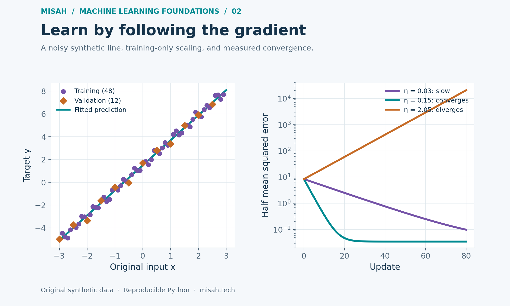
In part one, we found a regression line by solving a small algebraic problem. Many models are too large or complicated for that direct approach. Gradient descent offers a different route: begin with a guess, measure how the objective changes with each parameter, and take repeated steps toward a lower value. This lesson makes those derivatives visible before using them to fit data.

We will create a noisy synthetic relationship, reserve some observations for validation, check an analytic gradient against finite differences, and train a model from zero. All cells are self-contained and use the standard Python library. The dataset describes no real organization or experiment, and its small validation result is a teaching measurement rather than a performance claim.

1. A derivative describes a local change

For a scalar function, a derivative is the limiting rate of change near a point. A first-order approximation says that a small input change produces approximately the derivative times that change. With several parameters, collect the partial derivatives into a gradient. Its components tell us how sensitive the objective is to a small change in each coordinate while the other coordinates stay fixed.

The gradient points toward the steepest local increase under the ordinary Euclidean metric. Moving in its negative direction can reduce the objective when the step is sufficiently small. This is local information: a derivative does not tell us that an arbitrarily large jump will improve the result, and a low gradient alone does not prove useful predictions on unseen data.

2. Separate data before learning anything from it

Our sixty inputs run from −3.0 to 2.9. The target is a straight line with intercept 1.5 and slope 2.2 plus a small deterministic oscillation. Sine and cosine supply repeatable noise so the numerical experiment remains inspectable. This noise is constructed, not a claim that real measurement errors follow a periodic pattern.

Every fifth observation goes into validation; the other forty-eight are training observations. This interleaved split gives both groups coverage across the input interval. It is appropriate for illustrating bookkeeping in this constructed example, but would be misleading for a forecasting problem where later observations must remain strictly in the future. Split strategy must follow how examples become available.

We estimate the input mean and standard deviation using only training observations. Training and validation then use those same saved values. Let z be the standardized input and a its coefficient. This puts the input on a moderate numerical scale and helps us reason about the learning rate. Do not recompute a separate validation mean or let validation targets influence preprocessing.

3. Differentiate, then check the implementation

The one-half factor cancels the two from differentiating a square. For the intercept, every prediction changes at rate one; for the coefficient, each prediction changes at rate z. Applying the chain rule produces two averages. Both must be calculated using the same current parameters before either parameter is updated.

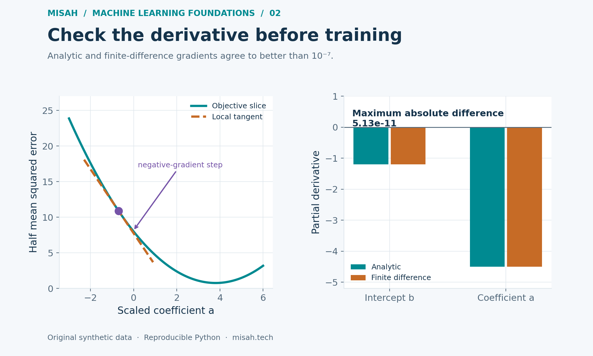
A finite-difference check compares these analytic derivatives with small numerical perturbations. We use a centered difference, evaluating the objective on both sides of the current value. The result should be close, not bit-for-bit identical: subtraction and floating-point rounding introduce error. An extremely tiny perturbation can make cancellation worse instead of making the estimate more accurate.

from math import sin, cos, sqrt

# Deterministic synthetic noise makes this experiment reproducible.
data = []
for i in range(60):
    x = (i - 30) / 10
    y = 1.5 + 2.2*x + 0.35*sin(1.7*i) + 0.12*cos(0.9*i)
    data.append((x, y))
train = [row for i, row in enumerate(data) if i % 5 != 0]
mean = sum(x for x, y in train) / len(train)
scale = sqrt(sum((x - mean)**2 for x, y in train) / len(train))
rows = [((x - mean) / scale, y) for x, y in train]

def loss(b, a):
    return sum((b + a*z - y)**2 for z, y in rows) / (2*len(rows))

b, a = 0.3, -0.7
errors = [b + a*z - y for z, y in rows]
analytic = [sum(errors)/len(rows),
            sum(e*z for e, (z, y) in zip(errors, rows))/len(rows)]
eps = 1e-5
numeric = [(loss(b+eps, a) - loss(b-eps, a))/(2*eps),
           (loss(b, a+eps) - loss(b, a-eps))/(2*eps)]
gap = max(abs(u-v) for u, v in zip(analytic, numeric))
print('analytic gradient:', [round(v, 6) for v in analytic])
print('finite differences:', [round(v, 6) for v in numeric])
print(f'maximum difference = {gap:.3e}')
print(f'training-only mean = {mean:.6f}; scale = {scale:.6f}')
assert gap < 1e-7

if 'plot' in globals():
    grid = [-5 + i*0.05 for i in range(201)]
    plot({'title': 'A slice through the squared-error objective',
          'xLabel': 'Scaled-feature coefficient a', 'yLabel': 'Half mean squared error',
          'series': [{'name': 'Loss with intercept fixed at 0.3', 'kind': 'line',
                      'points': [[v, loss(0.3, v)] for v in grid]}]})

The original cell checks the gradient at intercept 0.3 and scaled coefficient −0.7, far from the optimum. Its assertion requires the two methods to agree within 10⁻⁷. Checking only at the fitted solution would be less revealing, because near-zero derivatives can hide some implementation mistakes. Try another non-optimal parameter pair and keep the check in place.

4. Take repeated steps and record the objective

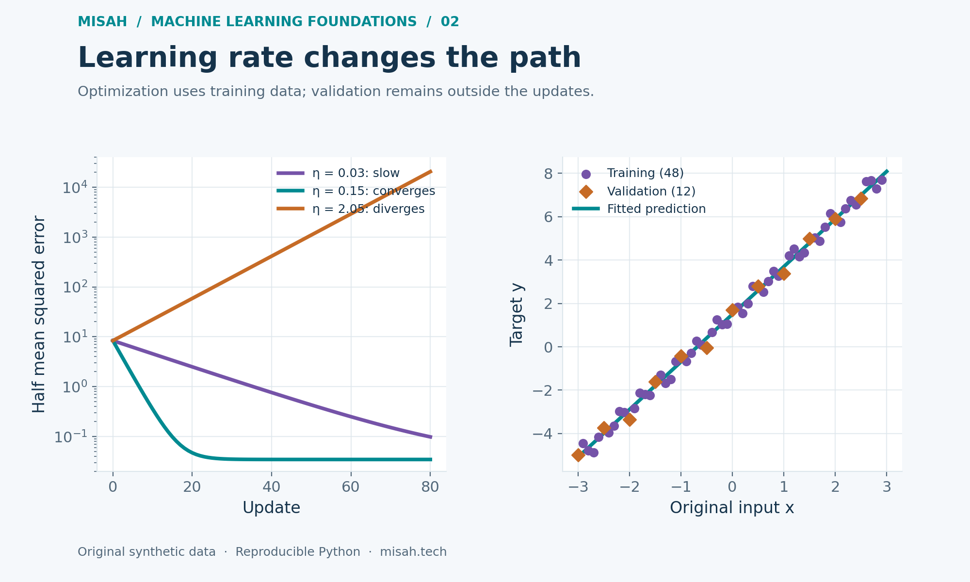
The next cell starts both parameters at zero and performs two hundred batch updates with learning rate 0.15. Batch means every training observation contributes to every update. We log the objective before the first update and after each subsequent update. Finally, we convert the coefficient and intercept back into the original input units so the fitted line can be interpreted alongside the generator.

from math import sin, cos, sqrt

# This cell repeats all setup: it does not depend on the preceding cell.
data = []
for i in range(60):
    x = (i - 30) / 10
    y = 1.5 + 2.2*x + 0.35*sin(1.7*i) + 0.12*cos(0.9*i)
    data.append((x, y))
train = [row for i, row in enumerate(data) if i % 5 != 0]
validation = [row for i, row in enumerate(data) if i % 5 == 0]
mean = sum(x for x, y in train) / len(train)
scale = sqrt(sum((x - mean)**2 for x, y in train) / len(train))
scaled = [((x - mean)/scale, y) for x, y in train]
b = a = 0.0
learning_rate = 0.15
history = []
for step in range(201):
    errors = [b + a*z - y for z, y in scaled]
    history.append([step, sum(e*e for e in errors)/(2*len(errors))])
    if step == 200:
        break
    db = sum(errors)/len(errors)
    da = sum(e*z for e, (z, y) in zip(errors, scaled))/len(errors)
    # Compute both gradients before changing either parameter.
    b -= learning_rate*db
    a -= learning_rate*da

slope = a/scale
intercept = b - a*mean/scale
def mse(rows):
    return sum((intercept + slope*x - y)**2 for x, y in rows)/len(rows)
baseline = sum(y for x, y in train)/len(train)
baseline_mse = sum((baseline-y)**2 for x, y in validation)/len(validation)
print(f'train = {len(train)}; validation = {len(validation)}')
print(f'intercept = {intercept:.6f}; slope = {slope:.6f}')
print(f'training MSE = {mse(train):.6f}; validation MSE = {mse(validation):.6f}')
print(f'validation MSE of training-mean baseline = {baseline_mse:.6f}')

if 'plot' in globals():
    plot({'title': 'Watch gradient descent reduce training loss',
          'xLabel': 'Update', 'yLabel': 'Half mean squared error',
          'series': [{'name': 'Training objective', 'kind': 'line', 'points': history}]})
    grid = [-3 + i*0.03 for i in range(201)]
    plot({'title': 'Keep validation observations outside fitting',
          'xLabel': 'Original input x', 'yLabel': 'Target y',
          'series': [
              {'name': 'Training data', 'kind': 'scatter', 'points': [list(r) for r in train]},
              {'name': 'Validation data', 'kind': 'scatter', 'points': [list(r) for r in validation]},
              {'name': 'Fitted prediction', 'kind': 'line',
               'points': [[x, intercept+slope*x] for x in grid]},
          ]})

5. Distinguish optimization from generalization

For this particular standardized single-input problem, the training mean of z is zero and its mean square is one. Consequently, the Hessian for parameters (b, a) is the identity up to rounding. Each error in a parameter is multiplied by 1 − η per update. A fixed learning rate between zero and two converges; 2.05 grows in magnitude. This unusually simple result does not supply a universal learning rate for other models.

Feature scaling changes the shape of the objective in parameter coordinates. With many inputs, correlations and unequal scales can produce narrow curved contours that slow simple gradient descent. Smaller steps, better scaling, line searches, or a different optimizer may help. None of these choices repairs an incorrect target, leaked preprocessing, or an evaluation set that does not resemble the deployment problem.

With the cell unchanged, the recovered original-unit intercept is 1.499235 and the slope is 2.196297. Training MSE is about 0.069408 and validation MSE is about 0.069389, compared with 14.515252 for the training-mean baseline on validation. These values are reproducibility checks for the specified data and split; changing the experiment should change the numbers.

The printed mean squared errors use the ordinary average of squared residuals, twice the objective plotted during training. Compare validation MSE with a baseline that always predicts the training-target mean. Beating that baseline on these twelve constructed observations confirms a limited fact about this example. Repeatedly choosing settings based on the same validation set would eventually require a separate final test set.

Try it yourself

• Change the learning rate to 0.03, then 2.05. Compare the numerical loss history with the convergence explanation before drawing conclusions from the fitted line.

• Remove standardization and compare the range of stable learning rates. Keep training and validation boundaries unchanged.

• Increase the synthetic noise amplitude. Explain why reaching the optimization minimum cannot force both training and validation MSE to zero.

• Replace the line with a curved target. Decide whether a lower training objective reflects a suitable model or only better optimization of a restricted model.

Sources and reproducibility

For descent directions, step sizes, and convex convergence reasoning, see Boyd and Vandenberghe’s unconstrained-minimization lecture. The identity-Hessian argument and all numerical experiments above are worked out specifically for this article’s data.

For the practical boundary between fitting preprocessing and transforming held-out data, see scikit-learn’s guidance on data leakage. The code does not require scikit-learn or any downloaded dataset.

Continue the foundations series

Part 1: Vectors, matrices, and linear regression

You are reading this part: Part 2: Calculus and gradient descent

Part 3: Probability and Bayes classification