Machine Learning Foundations 3: Probability and Bayes Classification

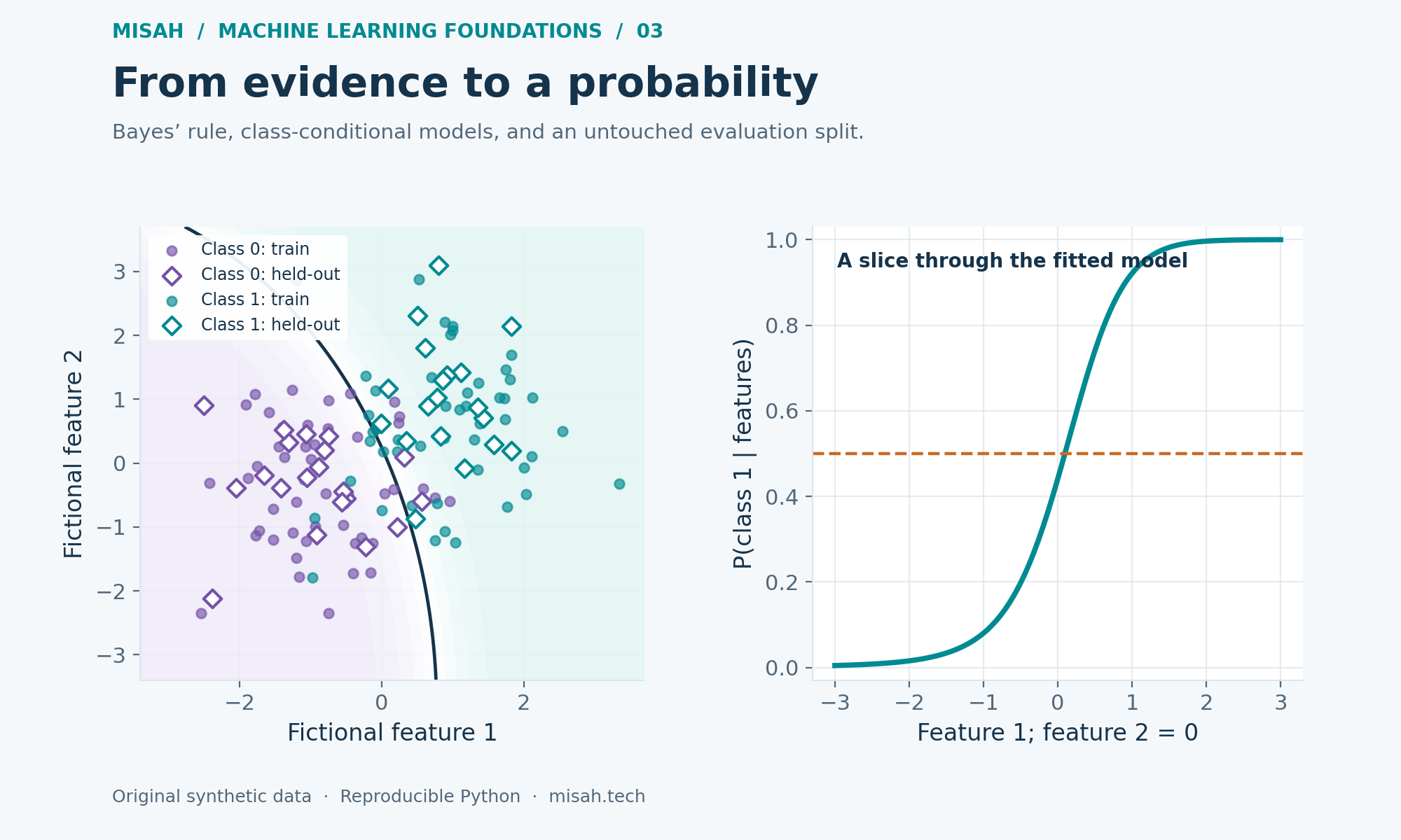
A regression model predicts a quantity. A classifier chooses among categories, often by estimating probabilities first. This final part of our Machine Learning Foundations series builds a probabilistic classifier from the ground up: begin with prior beliefs, update them using observations, perform the arithmetic in log space, and evaluate decisions on examples excluded from training.

We will use two fictional sensor features and synthetic classes zero and one. They have no medical, security, or business meaning. The goal is to inspect the mechanics of Gaussian Naive Bayes, including the assumptions that make it simple and the reasons its probabilities still deserve scrutiny. Each Python cell runs independently with no external packages or network requests.

1. Reverse a conditional probability carefully

Suppose ten percent of fictional messages contain an issue. A flagging rule catches eighty percent of those issues, but also flags twenty percent of messages without an issue. What fraction of flagged messages actually contain an issue? The answer is not eighty percent. That rate conditions on an issue already existing; our question conditions on observing a flag instead.

Think in expected counts per one thousand messages. One hundred contain issues, so eighty are flagged. Nine hundred do not contain issues, so one hundred eighty are flagged. Of the two hundred sixty total flags, only eighty concern an issue: approximately 30.77 percent. Expected counts make the denominator visible without changing Bayes’ rule.

# A fictional flagging rule; these rates are invented for the lesson.
prior_issue = 0.10
flag_given_issue = 0.80
flag_given_no_issue = 0.20

def posterior(prior):
    joint_issue_flag = flag_given_issue*prior
    flag_rate = joint_issue_flag + flag_given_no_issue*(1-prior)
    return joint_issue_flag/flag_rate

p = posterior(prior_issue)
print(f'issue-and-flag share = {prior_issue*flag_given_issue:.3f}')
print(f'flagged share = {prior_issue*flag_given_issue + (1-prior_issue)*flag_given_no_issue:.3f}')
print(f'P(issue | flagged) = {p:.6f}')
print('Expected counts per 1,000: 80 flagged issues and 180 flagged non-issues.')
assert abs(p - 80/260) < 1e-12

if 'plot' in globals():
    plot({'title': 'The same flag has different meaning at different base rates',
          'xLabel': 'Prior probability of an issue', 'yLabel': 'Probability of issue given a flag',
          'series': [
              {'name': 'Posterior after flag', 'kind': 'line',
               'points': [[i/100, posterior(i/100)] for i in range(1, 100)]},
              {'name': 'Our fictional base rate', 'kind': 'scatter', 'points': [[prior_issue, p]]},
          ]})

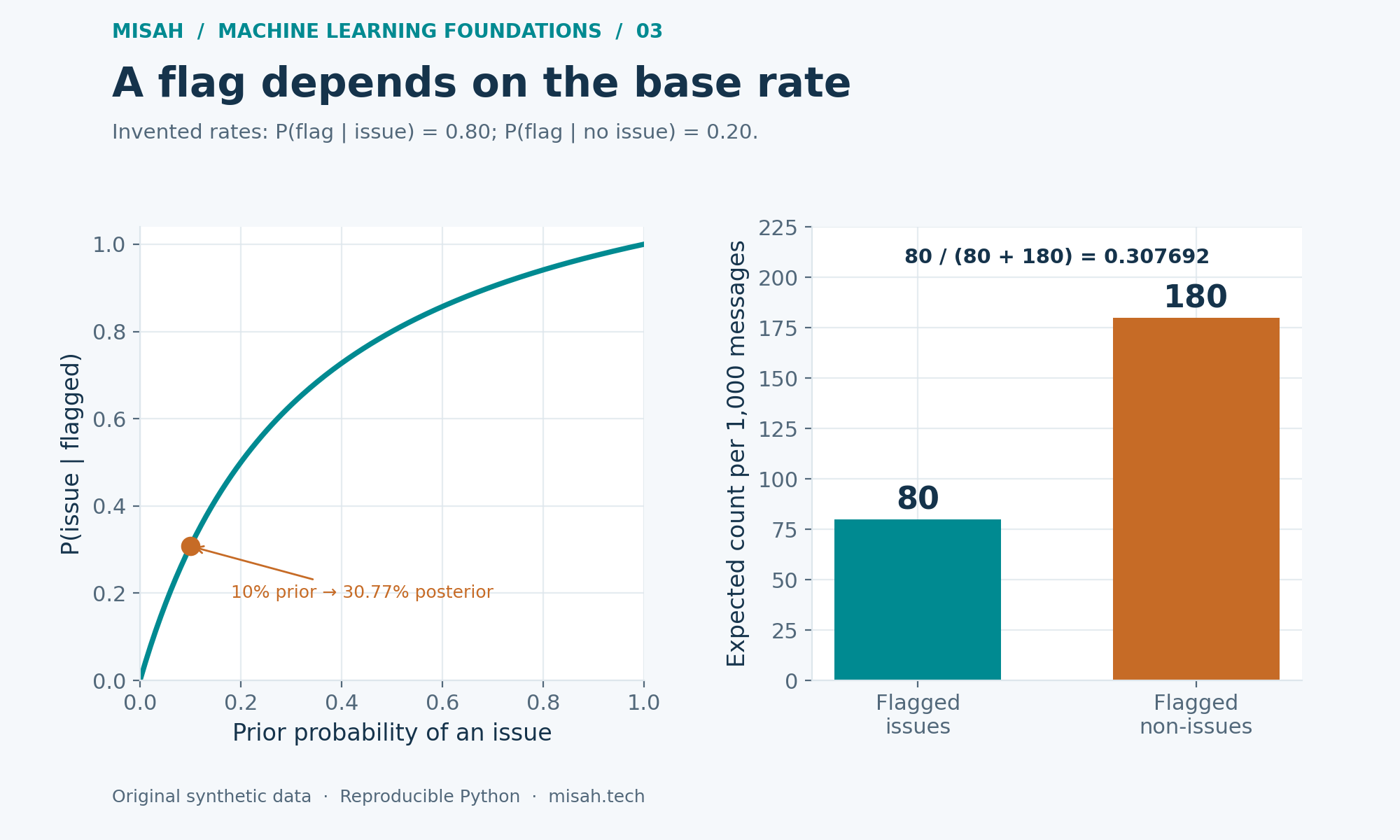
The prior is the probability before using the current observation. The likelihood describes how compatible the observation is with a class. The posterior combines them. Changing class prevalence can change the posterior even when the same observation has the same class-conditional likelihoods. A probability learned under one sampling process therefore needs care when moved to another population.

2. Turn several features into a tractable model

For continuous inputs, class-conditional likelihoods are probability densities. A density value is not the probability of observing one exact real number and can exceed one. Gaussian Naive Bayes models each feature with a normal distribution inside each class, then multiplies those densities. The “naive” assumption is conditional independence given the class, not unconditional independence across the whole dataset.

Our generator deliberately creates independent feature draws within each class, so the model family is well matched to the teaching problem. Real features often overlap or correlate. Two measurements of nearly the same quantity can make a naive model count similar evidence twice. Good classification accuracy on one dataset would not establish that the resulting probabilities are calibrated.

3. Estimate parameters from training observations only

We generate seventy examples per class. The first fifty from each class form one hundred training observations; the remaining forty total observations are held out. Because each draw comes from the same synthetic generator, this split is a convenient demonstration. For real grouped, temporal, or repeated measurements, independence between splits needs a more deliberate design.

These are maximum-likelihood Gaussian variance estimates with divisor n_c, rather than the n_c − 1 estimator often used for unbiased sample variance. We floor each variance at 10⁻⁶ to avoid division by zero. That floor is tied to feature units and is an explicit numerical guard for this example, not a generally optimal smoothing setting.

4. Add log likelihoods instead of multiplying tiny numbers

Products of many small densities can underflow to zero. Taking logarithms replaces multiplication with addition while preserving the largest score. For a class decision, the common evidence denominator can be omitted. For normalized probabilities, it must be restored. We subtract the largest log score before exponentiating, which avoids unnecessarily large exponentials and gives an elementary log-sum-exp calculation.

Read the following cell in three passes: first the generator and split, then parameter estimation, then probability calculation and evaluation. Box–Muller turns uniform pseudo-random draws into normal draws; the fixed seed makes our original example reproducible. No held-out label influences the means, variances, or priors. The assertion checks that every returned probability pair sums to one within rounding tolerance.

from math import log, exp, sqrt, cos, pi
from random import Random

# Two fictional sensor features; all 140 observations are generated here.
rng = Random(41)
def normal():
    # Box-Muller transform of two uniform pseudo-random numbers.
    return sqrt(-2*log(max(rng.random(), 1e-12)))*cos(2*pi*rng.random())

train, heldout = [], []
for label, center, spreads in [(0, (-0.9, -0.4), (0.9, 0.85)),
                                (1, (0.9, 0.7), (0.9, 1.0))]:
    for i in range(70):
        x = [mu + sd*normal() for mu, sd in zip(center, spreads)]
        (train if i < 50 else heldout).append((x, label))

model = {}
for label in (0, 1):
    rows = [x for x, y in train if y == label]
    means = [sum(x[j] for x in rows)/len(rows) for j in range(2)]
    variances = [max(1e-6, sum((x[j]-means[j])**2 for x in rows)/len(rows))
                 for j in range(2)]
    model[label] = (len(rows)/len(train), means, variances)

def probabilities(x):
    scores = []
    for label in (0, 1):
        prior, means, variances = model[label]
        score = log(prior) - 0.5*sum(
            log(2*pi*v) + (value-mu)**2/v
            for value, mu, v in zip(x, means, variances))
        scores.append(score)
    peak = max(scores)
    weights = [exp(score-peak) for score in scores]
    return [weight/sum(weights) for weight in weights]

confusion = [[0, 0], [0, 0]]  # rows = truth; columns = prediction
brier = 0.0
for x, truth in heldout:
    p = probabilities(x)[1]
    prediction = int(p >= 0.5)
    confusion[truth][prediction] += 1
    brier += (p-truth)**2
tn, fp = confusion[0]
fn, tp = confusion[1]
accuracy = (tn+tp)/len(heldout)
precision = tp/(tp+fp) if tp+fp else 0.0
recall = tp/(tp+fn) if tp+fn else 0.0
print(f'training = {len(train)}; held-out = {len(heldout)}')
print('confusion matrix [truth rows, prediction columns]:', confusion)
print(f'accuracy = {accuracy:.3f}; class-1 precision = {precision:.3f}; recall = {recall:.3f}')
print(f'held-out Brier score = {brier/len(heldout):.6f}')
print('P(class 1 | features [0, 0]) =', round(probabilities([0, 0])[1], 6))
assert all(abs(sum(probabilities(x))-1) < 1e-12 for x, y in heldout)

if 'plot' in globals():
    series = []
    for rows, split in [(train, 'Training'), (heldout, 'Held-out')]:
        for label in (0, 1):
            series.append({'name': f'{split}, class {label}', 'kind': 'scatter',
                           'points': [x for x, y in rows if y == label]})
    plot({'title': 'Two synthetic features and an untouched held-out split',
          'xLabel': 'Fictional sensor feature 1', 'yLabel': 'Fictional sensor feature 2',
          'series': series})
    grid = [-3 + i*0.05 for i in range(121)]
    plot({'title': 'A probability slice, keeping feature 2 fixed at zero',
          'xLabel': 'Feature 1; feature 2 = 0', 'yLabel': 'P(class 1 | features)',
          'series': [{'name': 'Gaussian Naive Bayes', 'kind': 'line',
                      'points': [[x, probabilities([x, 0])[1]] for x in grid]}]})

5. Read more than one evaluation number

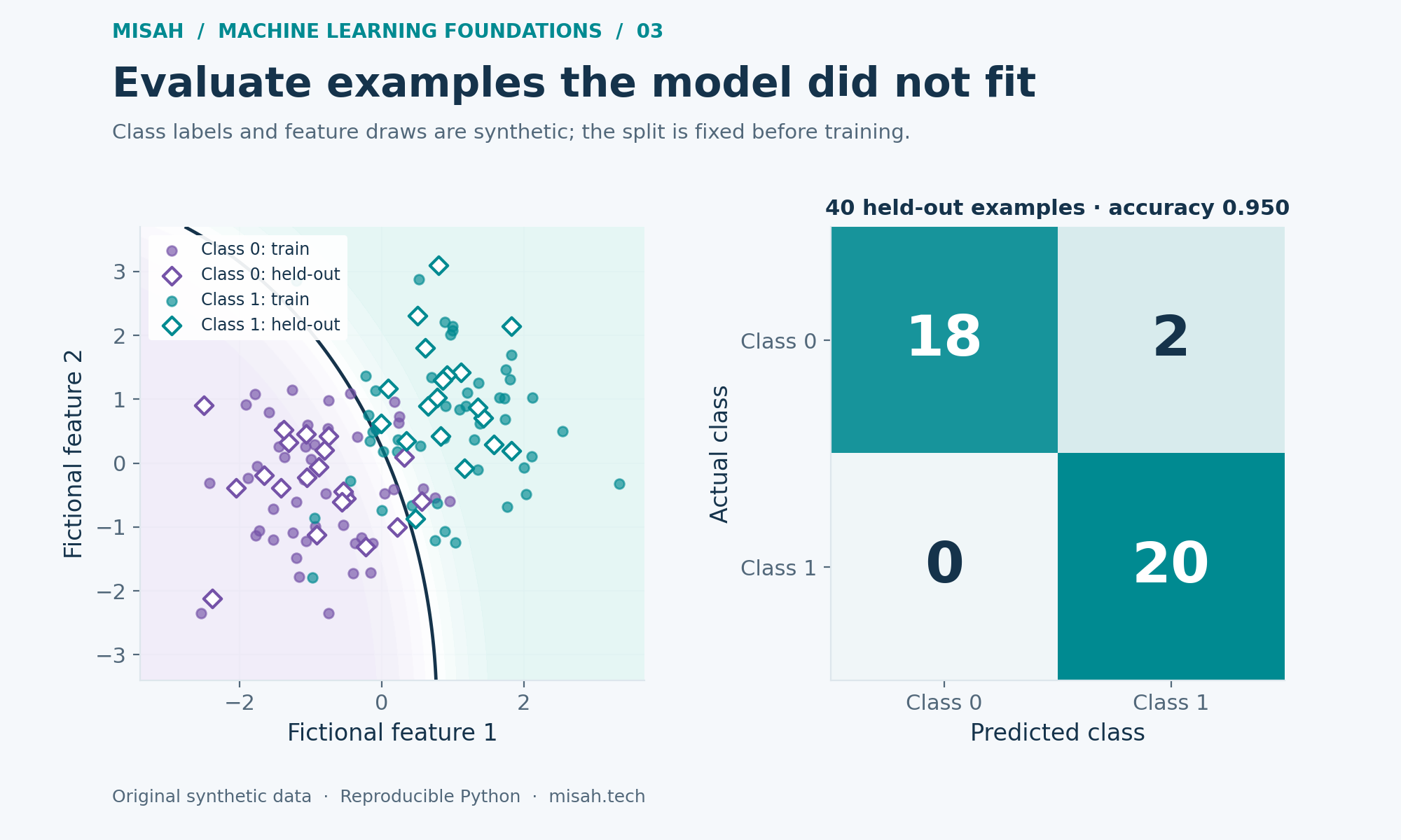
The confusion matrix puts true classes on rows and predicted classes on columns. For class one, true positives are correctly predicted ones, false positives are zeros called ones, and false negatives are ones called zeros. Accuracy counts all correct decisions; precision asks how many predicted ones were correct; recall asks how many actual ones were found. The code uses a probability threshold of one half.

For the fixed seed, the confusion matrix is [[18, 2], [0, 20]]. Accuracy is 0.950, class-one precision is approximately 0.909, and recall is 1.000; the Brier score is approximately 0.041887. There are only twenty held-out examples from each class. Two additional mistakes would noticeably change these rates, so avoid reading more certainty into them than the sample supports.

The Brier score evaluates probabilities rather than only thresholded labels. Lower is better on a fixed dataset, but one small score does not prove calibration or robustness. A constant probability of one half has Brier score 0.25 on these binary labels, providing a simple reference. If classification costs differ, the threshold should reflect those costs and be chosen without tuning against the final held-out set.

The probability slice in the cell fixes feature two at zero while moving feature one. It is one cross-section through a two-dimensional model, not a complete picture of every possible input. Predictions far outside the training clouds rely heavily on the assumed Gaussian tails. A very confident extrapolation can still be wrong when the model assumptions stop describing the world.

Try it yourself

• Change the class frequencies and compare learned priors with the earlier base-rate example. Keep a record of which population the held-out split represents.

• Make the two features strongly correlated within each class. Inspect both thresholded errors and probability scores; ask what evidence is being counted twice.

• Increase the overlap between class centers. Explain why a correctly implemented model can still have unavoidable errors on overlapping synthetic distributions.

• Try a different decision threshold without refitting. Identify which confusion-matrix counts change, and preserve a fresh evaluation set if you select the threshold using labels.

Sources and reproducibility

The standard conditional-independence model and Gaussian class-conditional density are documented in scikit-learn’s Naive Bayes guide. All synthetic data, numerical checks, and visualizations in this article are original.

For the logarithm, exponential, square root, and trigonometric functions used in the implementation, see Python’s math documentation. We use these elementary operations directly to keep every part of the classifier inspectable.

For definitions of the decision and probability metrics used above, see scikit-learn’s model-evaluation guide. Our Brier calculation uses the binary convention: the mean squared error of the probability assigned to class one.

Continue the foundations series

Part 1: Vectors, matrices, and linear regression

Part 2: Calculus and gradient descent

You are reading this part: Part 3: Probability and Bayes classification